

Advancing scientific excellence by publishing influential results in fundamental, applied, and interdisciplinary physics across @apsphysics' journals.
- Tweets435
- Following5
- Followers1.2K
- Likes74






ALT A diagram showing how programmable optical lattice control works over time. Atoms occupy neighboring wells in a 1D lattice, shown as particles sitting in a repeating series of double-well potentials. Over time, neighboring site pairing alternates between two configurations, allowing different atoms to interact. Arrows between wells represent controlled tunneling and local energy offsets adjust the phase at individual sites. Insets illustrate an X rotation (produced by tunneling between two wells) and a Z rotation (produced by shifting the potential of one site).

ALT An image taken by the Hubble Space Telescope shows a galaxy cluster — bright specks and smears of light over the dark background of space — with a blue gas-like haze around the image. The blue is photons from the cosmic microwave background undergoing a boost of energy.

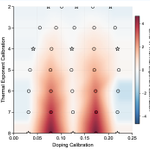
ALT Graph plotting doping calibration on the x-axis and thermal exponent calibration on the y-axis. It shows the error in an AI omnimeter as it estimates temperature-related values at left and doping at right for different simulated conditions. Circles and stars mark tested points, with stars indicating conditions included in training. Most of the plots are light-colored, representing small errors, while darker bands show larger errors the unseen doping levels. This shows that AI can estimate temperature and doping accurately across much of the tested range, including many conditions it wasn’t directly trained on.

ALT Graph plotting doping calibration on the x-axis and thermal exponent calibration on the y-axis. It shows the error in an AI omnimeter as it estimates temperature-related values at left and doping at right for different simulated conditions. Circles and stars mark tested points, with stars indicating conditions included in training. Most of the plots are light-colored, representing small errors, while darker bands show larger errors the unseen doping levels. This shows that AI can estimate temperature and doping accurately across much of the tested range, including many conditions it wasn’t directly trained on.

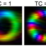
ALT Two images showing sound pressure field distributions of perfect ST acoustic vortices with topological charges 𝑙 = 1 on the left and 𝑙 = 5. Brightness represents the amplitude and hue represents the phase.

ALT A schematic labeled CF-Flow: Composite-fermion wavefunctions with backflow. At the left, a blue sphere surrounded by red arrows indicating an outward magnetic field contains three yellow dots labeled r1, r2, and r3. Their positions feed into an AI model, represented by a circuit-patterned brain, which produces a wavefunction correction and new backflow coordinates. On a blue sphere at the right, yellow arrows connect the faded original positions to new positions labeled R1, R2, and R3. The diagram illustrates how CF-Flow builds on known physics to model the effects of interactions.

ALT UN’s SDG logo. “SUSTAINABLE DEVELOPMENT GOALS” in large blue letters. The “O” in “GOALS” is a multicolored wheel.
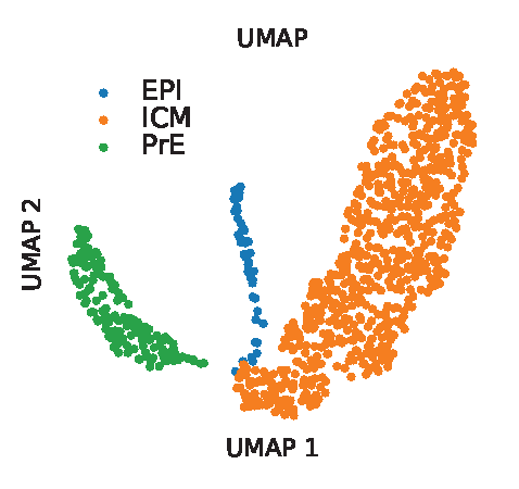
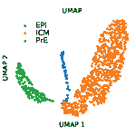
ALT Scientific figure modeling a bifurcation of the mouse gut endoderm in early embryo development using uniform manifold approximation and projection (UMAP) visualization. The inner cell mass or ICM (represented by orange dots) can differentiate into epiblast cells or EPI (blue dots) and primitive endoderm cells or PrE (green dots). The model dynamics were inferred by matching between cells from embryonic days E3.5 to E4.5 using optimal transport.

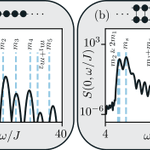
ALT A side-by-side comparison of an Ising chain (left) and a weakly coupled Ising ladder (right). Black curves show the measured excitation spectra with vertical blue, dashed lines marking the particle masses predicted by E8 and D8(1) symmetries. Above each graph, black dots depict the atomic geometries: a single row for the chain and two connected rows for the ladder. The plots show how coupling the chains reorganizes the excitation spectrum.

ALT A series of fluorescence microscopy images of microtubule bundles coated with condensed microtubule-associated proteins at 2,000 nanomolar. They appear as glowing neon streaks on black backgrounds. Two panels at the top show BuGZ in teal and microtubules in magenta, showing BuGZ droplets and films along the bundles in merged images. Two lower panels show TPX2 lime green and microtubules in magenta, with similar droplet and film structures visible again in merged images. These enlarged views show how condensates appear to bridge or coat microtubules, which makes sense if bundling is driven by capillary forces. Scale bars are labeled 1 micrometer.

ALT Diagrams comparing two kinds of quantum operator spreading. On the top, dots in ovals show an operator spreading across different parts of a physical system. On the bottom, it spreads through a much larger spherical space of possible operators. The figure shows that quantum chaos can involve both kinds of spreading.

ALT This is a series of four graphs showing what happens to pollination modes during pollen limitation. In general, there is significant expansion in the parameter region showing full self-incompatibility is favored. Meanwhile, the region exhibiting the mixed phase shrinks. The top two graphs, marked a and b, map the mean and standard deviation of the self-incompatible population fraction. The bottom two graphs represent the mean and the coefficient of variation, or the ration of standard deviation to mean.

ALT A graph comparing two ways to calculate a small energy contribution in diamond. An orange curve labeled SOS (sum over state) rises toward a black dashed line labeled DFPT (density functional perturbation theory) as more electronic states are included. Both methods approach the same result (about 3.6 meV per unit cell), showing that the calculation is reliable.

ALT A graph comparing the infrared spectrum of protonated oxalate measured experimentally with spectra calculated using two machine-learning models, PIP-PES and PhysNet, across frequencies of about 900–3,500 cm-1. The spectra have closely matching peaks, and a difference line shown in between them is practically flat, showing a very strong agreement between the models.

ALT Schematic showing the algorithm for constructing gapped boundaries of a topological generalized Pauli stabilizer code. The diagram flows from top left to top right, then bottom left to bottom right. It begins with a grey plane with repeated purple code on it. It is truncated–depicted by cutting the plane and code with scissors. Numerous operations follow, depicted by a series of arrows and images of computers, introducing boundary gauge operators (purple and green symbols) and then the identification of boundary string operators and boundary anyons (a string of orange lines marked X, bounded by the letters a and a-1 and a red line with multiple z’s marked along it, bounded by the letters b and b-1). The bottom row shows topological spin and braiding statistics (rearranging the red and orange lines), then boundary anyon condensation to create short boundary string operators and topological order completion to construct the gapped boundary Hamiltonian, with a spark of energy violation.

ALT A top-down structural view of a bacterial flagellar motor, which looks somewhat like a sunflower with short petals. Concentric rings, each with repeating patterns, are shown with labeled components including the FlgG ring in the center, the LP- ring outside of that, and the C- and MS- rings on the outer edge. An arrow shows counter-clockwise rotation in the middle and other arrows represent torques acting on the motor, labeled fdr, fop, and f.

ALT A figure titled “Setting Up the Problem.” A black line with arrows goes from left to right representing a black hole’s path, with a shaded circle (the black hole) in the middle. A red squiggly line representing an incoming gravitational wave approaches the circle from the upper left, then another red squiggly line representing an outgoing gravitational wave exits the circle moving to the upper right. The change in direction represents the gravitational wave scattering off the black hole.

ALT A view of Earth from space with a network of interconnected lines and nodes surrounding the planet, symbolizing global communication or connectivity. Sunlight is visible, illuminating part of Earth. The background is a dark, starry space.

ALT An illustration of the photon counter and its detection sequence. At the top, a simple diagram displays the three motions in the Penning trap involving the axial, modified cyclotron, and magnetron components, indicated as three points along a red circle. At the bottom is a cross-sectional view of the trap (yellow rectangle) and its electronic detection circuit diagram.